An Alien Landscape
Find The Lowest Point
Coordinates in the mb-plane
Lines in the xy-plane

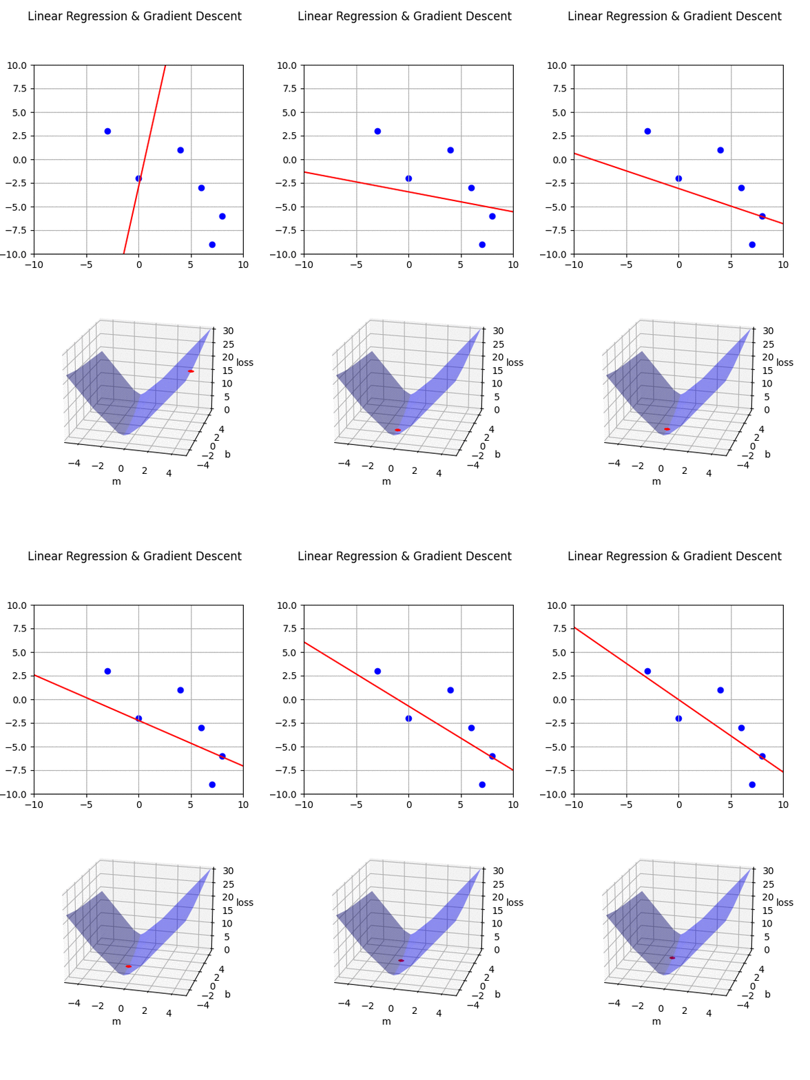
Gradient Descent and Linear Regression

This project describes the mathematics behind machine learning and AI. Gradient descent is the process by which model weights and biases are adjusted when training neural networks.

An Alien Landscape

Imagine yourself standing on the surface of an alien planet. It is a desolate surface with no liquid water, and no visible light from any source. As you stand on the surface, you can feel the slope of the ground under your feet, but you can not see the terrain around you because there is no light.

The gravity is weak on this planet, and you are able to jump enormous distances, like the Disney hero John Carter.

You know that the surface of this planet has peaks and valleys, but you don't know where they are. Your only tool for navigation is a GPS unit that displays your longitude, latitude, and elevation.

You have one objective: you must find the lowest point of elevation on the planet.

The only information you have comes from the slope of the ground beneath your feet and your GPS unit (longitude, latitude, and elevation). The only transportation you have is your ability to step, or jump, any distance you'd like in any direction you choose.

This is the challenge presented by gradient descent. How do you find the lowest point of elevation on a surface?

Find The Lowest Point

The most common approach to this problem is to use the following process:

1. Pick an arbitrary distance to use as your "learning rate". This learning rate will be used as a factor in determining how far you will jump for every iteration of the gradient descent process. For this example, the learning rate will be 2 km.

2. Find the slope of the surface beneath your feet. When gradient descent is implemented mathematically, this is calculated by finding the partial derivative along each axis of the surface. But for our example you can imagine some tool that measures the magnitude and direction of the slope of the ground that you are standing on. For example, you might find a slope with a magnitude of 5 in the northeast direction.

3. Move a distance that is equal to your learning rate * the magnitude of the slope vector in the downhill direction. So in our example this would result in jumping 10 km southwest (northeast is uphill in our example because the slope is positive in that direction).

4. Check the elevation at your new location after moving, and repeat steps 2-4.

You can imagine how this process might look after a few iterations. Each iteration changes your coordinates and moves you in the downhill direction. However you might find that your elevation increases after some iterations when a slope is so steep, or a learning rate so high, that you jump over a valley and end up at a higher point on the other side of it.

It's important to note that this process is good for finding a local minimum (e.g. on earth, this could be somewhere like Death Valley), but is not garunteed to find the absolute minimum (e.g. the Mariana Trench).

Coordinates in the mb-plane

In fact, gradient descent is even simpler than the scenario I just described, because rather than dealing with a spherical surface of a planet, our surface extends along a plane. Like a flat earth. This means that instead of having a spherical surface with a finite area, we have a surface that extends to infinity in every direction (north, south, east, and west).

Now, we should start being more specific about what exactly is happening mathematically, so we will parameterize our surface in 3D space. It would be simplest to call these axes (x,y,z) where (x,y) are our coordinates and z is our elevation. However, we will be using the xy-plane for something else in the next step, so instead let's parameterize this space using (m,b,z) where (m,b) are our coordinates and z is our elevation.

This would mean that north and south are +b and -b. Likewise, east and west would be +m and -m. Our surface would be defined as z = f(m,b) and it would extend to infinity in every direction along the mb-plane.

In this example f(m,b) is our loss function (sometimes called an error or cost function). The loss function can be used to calculate our elevation, z, at any point on the mb-plane. Our elevation indicates how well a line in the xy-plane, y = mx + b, fits a dataset of (x, y) coordinate pairs. This is why we are looking for the lowest point of elevation. The coordinates (m, b) at the lowest point of elevation would define the line of best fit, y = mx + b, for our dataset.

Your coordinates in the mb-plane define a line in the xy-plane

Let's connect this gradient descent process that exists in the 3D space (m,b,z) to a line in the xy-plane. A line on the xy-plane is often defined using the slope-intercept form of y = mx + b, where m is the slope and b is the y-intercept. Any non-vertical line on the xy-plane can be described using this form, by setting different values for m and b.

This connection between our coordinates on the surface, (m, b), and a line in the xy-plane, y = mx + b, is the most important thing to understand because it drives the whole process.

This is why we parametrized the surface coordinates using m and b. Every point on the surface has a unique combination of the coordinates m and b, so every point on the surface represents a unique line in the xy-plane.

If you walk east or west on the surface (+m or -m), then the slope of the line in the xy-plane changes. If you walk north or south on the surface (+b or -b) then the line shifts up or down along the y-axis. So the jump 10km southwest in our example would have changed both the slope and the y-intercept on the line represented by our coordinates on the surface.

You can click and drag on the mb-plane below to see how the corresponding line changes on the xy-lane.

mb-plane (click to change m, b)

m = 0, b = 0 → y = 0x + 0